Essential Excel: The Powerful INDEX & MATCH Functions in Excel.
The Index & Match Function:
The INDEX Function can return an item from a specific position in a table.
The MATCH Function returns the relative row position of a value in a list.
The INDEX and MATCH Functions are often used together, as a flexible and powerful tool for extracting data from a table.
The VLOOKUP Function can only search the leftmost column of your table and search from left to right.
But what happens if you want to search the third column of your table and search from right to left. We can achieve this by using the INDEX and MATCH Functions together.
INDEX Function — Arguments
The INDEX function has three arguments
- Array: Where is the list? If you use an Absolute Reference ($A$2:$B$4), instead of a Relative Reference (A2:B4), it will be easier to copy to formula to other cells. Or, Name the lookup table, and refer to it by Name.
- Row_num: Which row has the value you want returned?
- [Column_num]: Which column has the value you want returned?
INDEX Function – Examples
Our table of data is $D$2:$H$7. I can access the content of any of the cells in this table by using the INDEX Function.
As per screenshot above,
=INDEX($D$2:$H$7,2,2)
means go to the range D2:H7, then go row 2 and then column 2 and return the value in this cell.
Important Note:
When counting the rows and columns, it has nothing to do with the spreadsheet rows and columns, but the rows and columns relative to the table.
You count the rows and column relative to how the table was defined.
For example is ‘Michael’ on row 1 or row 2. The answer to that depends on how the table was defined. In our example, the table was defined as D2:H7, so ‘Michael’ is on row 2.
You could have defined the table without including the headers i.e.
D3:H7, then ‘Michael” would be row 1.
The Important MATCH Function:
The Match Function allows you search a given column to find the relative position of the first occurrence of a text string or number.
Repeat: It does not return the absolute row reference but that relative to that column.
Syntax
=Match (lookup_value, lookup column range, match type)
While the Lookup functions gives you the value in a specific cell, use MATCH to find the RELATIVE position of a value in a column range.
Last argument 0 gives first exact match.
MATCH FUNCTION EXAMPLES:
As in screenshot, =MATCH(290,$H$3:$H$7,0) means look for the value ‘290’ in the column range H3:H7.
So MATCH Function will look in row 1 of that column range which is H3.It’s not in that cell, so then it looks in H4. It finds it. 290 is in row 2 of the defined column range H3:H7
Note =MATCH(412,F2:F7,0)
This is giving the answer 3 because we defined the range as including the header, so therefore the header is row 1.
Index and Match Functions Combined. An Example:
One advantage of the INDEX/MATCH Functions is that the lookup value can be in any column in the array, unlike the VLOOKUP Function, in which the lookup value must be in the leftmost column of the defined table.
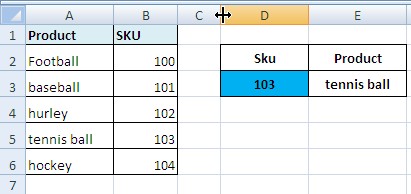
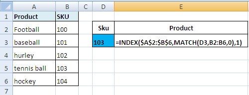
In A2:B6 range we have a list of products and their SKU numbers.
In Cell D3, I want to be able to type in any SKU and have its description appear in E3.
In this situation, I can’t use the VLOOKUP Function, because the column I am searching is not the left- most and I need to search from right to left. So how will I solve this problem.
Well I know the location table I want to search and I know that the Product name will be somewhere in the first column of that table. The only unknown part of the jigsaw is the relative row position of the SKU I am looking for.
If I knew that, I could use the INDEX Function to bring back the required value.
But hold on, I could use the MATCH Function to find this relarive Row position. So to find SKU 103 use
MATCH(D3,B2:B6,0) which returns 4
We can then combine this with the INDEX Function
=INDEX($A$2:$B$6,MATCH(D3,B2:B6,0),1)
INDEX and MATCH — Example 2
The MATCH Function can be used to return values for both the row_num and column_num arguments in the INDEX function.
Set up the worksheet as shown at right
- Enter the following formula in cell C7: =INDEX($B$2:$D$4,MATCH(B7,$A$2:$A$4,0),MATCH(A7,$B$1:$D$1,0))
- Press the Enter key to see the result.
- The first MATCH function, MATCH(B7,$A$2:$A$4,0), returns 3, which is the position of "Pants" in the Items list.
- The second MATCH function, MATCH(A7,$B$1:$D$1,0), returns 2, which is the position of "Med" in the Size list.
- Then, the INDEX function, INDEX($B$2:$D$4,3,2), returns "30", which is the third item in the second column in the range $B$2:$D$4
|
|
A |
B |
C |
D |
|
1 |
|
Small |
Med |
Large |
|
2 |
Sweater |
10 |
12 |
15 |
|
3 |
Jacket |
30 |
35 |
40 |
|
4 |
Pants |
25 |
30 |
35 |
|
5 |
|
|
|
|
|
6 |
Size | Item | Price | |
|
7 |
Med | Pants |
? |


