Offset Function

This article will focus on the use of the OFFSET function and we promise to make you an expert in all tricks related to this useful Function.

In it’s simplest form,the OFFSET Function returns the value contained in a cell that is a certain number of rows and columns away from a base cell. Sounds complicated?

Let’s use an example to explain.

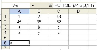
In the above diagram, cell A6 contains the character “a”.

If you look at the formula bar, you will notice that the character “a” was not typed into the cell. Instead, it was a result returned by the OFFSET Function.

We have basically instructed Excel to return the value that is found in cell A3.

How was this done?

1. First, we identify a cell as a starting point. This is our base cell. In the formula above, the base cell is A1 in “=OFFSET(A1,2,0,1,1)”

2. We have indicated in the formula that we want the result that is 2 rows below the base cell A1 “=OFFSET(A1,2,0,1,1)”

3. Next, we also tell the OFFSET Formula that the result should be 0 column from the base cell. By now, the formula would have identified that we are looking at the cell A3, which is 2 rows below A1 and zero column to the right of A1.

4. Finally, we told Excel that the size of the range we want is 1 row tall and 1 column high, i.e. a single cell “=OFFSET(A1,2,0,1,1)”

5. As a result of this instruction, the character “a” was displayed in cell A6.

Notes: a) If you want the OFFSET Function to move above the base cell, then enter it as a negative number. In the above example, the offset will return an error because it is unable to find anything above the cell A1 (outside the boundary of the excel worksheet). However, if you have entered the base cell as B3, then you could instruct the OFFSET Formula to move 1 row above the base cell.

The offset function will return the value “65” as its result. The formula to do this is “=OFFSET(B3,-1,0,1,1)”

b) The minimum number of cells to return is 1 as in this example “=OFFSET(A1,2,0,1,1)” is 1 row tall and 1 column wide. In this example, only 1 row and 1 column can be used in any container Function that the OFFSET Function might feed.

The size of the range can be increased, only when it is used together with another function, e.g. SUM , AVERAGE Functions etc Otherwise, it will return with an “#Value!” error.

C).The real power of the OFFSET function is that you can use other functions for some of the arguments.

If either of the “rows”, “columns”, “height” or “width” components are left blank, Excel will assume its value to be zero. For example, if the formula is written as OFFSET(C20, , 1, , ) Excel will see this as OFFSET(C38, 0, 1, 0, 0). But since “height” and “width” can be left out, therefore it can be typed as OFFSET(C20, , 1) since can be omitted.

Excel excludes the reference cell when calculating the “rows” and “columns” components. its like counting from 0,1,2 etc but includes the reference cell when calculating the “height” and “width” components.

Using Offset function in a SUM Function.

If we increase either the row height or column width in the OFFSET Function “=OFFSET(A1,2,0,1,1)” to more than 1, the reference is converted to a range.

In this section, we will explain how we make use of the OFFSET Function to find out sum of the range C1:C2 1.Set up the OFFSET Function such that it is referenced to the cell C1.

The formula will start with the base cell A1 “=OFFSET(A1,0,2,1,1)”.

Then, enter the number 0 to instruct the function to stay in the same row 1 “=OFFSET(A1,0,2,1,1)”.

Now we type 2 to indicated that we want to move 2 columns to the right of the base cell A1 “=OFFSET(A1,0,2,1,1)”

Please note that Column A is numbered 0.

Keep the last two numbers as 1 to indicate that we want the offset function to point to one single cell C1 “=OFFSET(A1,0,2,1,1)”. The result will show the value in cell C1, i.e. the number 43. 2. Now enclose the OFFSET Function within a container ffunction like SUM. =SUM(OFFSET(A1,0,2,1,1))

The result continues to show 43. 3. Since we want to sum the range C1:C2, we need to increase the row height to 2 =SUM(OFFSET(A1,0,2,2,1)) The number now changes to 75. It has included the number 32 in cell C2. The number 75 is the result of summing cell C1 (43) and C2 (32). See screenshot below.